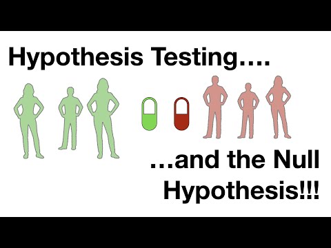
Introduction: Moving from Heuristics to Scientific Proof
In data science, observing an apparent pattern or numerical difference in sample data is never sufficient to justify business or scientific decisions. If users exposed to a new recommendation algorithm generate $4.2%$ higher revenue than users on the baseline algorithm, is that difference genuine, or is it merely random sampling noise? Statistical Hypothesis Testing provides the rigorous mathematical framework needed to make objective, reproducible decisions under uncertainty.
By defining null and alternative hypotheses, calculating test statistics, and comparing observed outcomes against theoretical sampling distributions, data scientists quantify the probability of empirical observations and establish statistically sound decision rules.
Core Concepts: The Hypothesis Testing Architecture
Every formal hypothesis test follows a standardized 5-step mathematical procedure:
- State the Null ($H_0$) and Alternative ($H_1$) Hypotheses:
- Null Hypothesis ($H_0$): The default proposition that there is no true effect, no difference between groups, or no relationship between variables.
- Alternative Hypothesis ($H_1$): The claim the researcher seeks to establish—that an effect, difference, or relationship exists.
- Specify the Significance Level ($alpha$): The probability threshold for rejecting the null hypothesis when it is actually true (Type I error rate). Industry standard is set to $alpha = 0.05$ (5%).
- Compute the Test Statistic: A standardized numerical value calculated from sample data that measures the degree of departure from $H_0$.
- Calculate the $p$-value: The probability of observing a test statistic at least as extreme as the one calculated, assuming that the null hypothesis is true:
$$ptext{-value} = P(text{Test Statistic} ge t_{obs} mid H_0)$$ - Formulate Decision Rule:
- If $ptext{-value} le alpha$: Reject $H_0$; the finding is statistically significant.
- If $ptext{-value} > alpha$: Fail to reject $H_0$; insufficient evidence exists to claim an effect.
Deep Dive: Decision Errors and Statistical Power
Because statistical decisions are made using samples rather than entire populations, two fundamental error states can occur:
| Statistical Decision | $H_0$ is Actually True (No Effect) | $H_0$ is Actually False (Real Effect) |
|---|---|---|
| Reject $H_0$ (Claim Effect) | Type I Error (False Positive) Probability = $alpha$ (typically 5%) |
Correct Decision (True Positive) Probability = $1 – beta$ (Statistical Power) |
| Fail to Reject $H_0$ (No Claim) | Correct Decision (True Negative) Probability = $1 – alpha$ (95%) |
Type II Error (False Negative) Probability = $beta$ (typically 20%) |
Statistical Power ($1 – beta$): The sensitivity of an experiment to detect a real effect of a given magnitude. Power is governed by four interdependent variables: sample size ($N$), effect size (Cohen’s $d$), significance level ($alpha$), and data variance ($sigma^2$). Increasing sample size is the most reliable way to boost statistical power.
Practical Code Demonstration: Testing in Python (SciPy)
import numpy as np
import scipy.stats as stats

# Scenario: Testing whether a new checkout layout increases revenue per user
np.random.seed(42)
control_group = np.random.normal(loc=50.0, scale=12.0, size=250)
treatment_group = np.random.normal(loc=53.5, scale=12.0, size=250)

# Check normality assumption: Shapiro-Wilk Test
stat_c, p_norm_c = stats.shapiro(control_group)
stat_t, p_norm_t = stats.shapiro(treatment_group)
print(f"Normality p-values: Control={p_norm_c:.4f}, Treatment={p_norm_t:.4f}")

# Check variance homogeneity: Levene's Test
stat_var, p_var = stats.levene(control_group, treatment_group)
print(f"Equal Variance p-value: {p_var:.4f}")

# Execute Two-Sample Independent t-Test (Welch's t-test doesn't assume equal variance)
t_stat, p_val = stats.ttest_ind(treatment_group, control_group, equal_var=False)

print(f"
Welch's t-statistic: {t_stat:.4f}")
print(f"p-value: {p_val:.6f}")

alpha = 0.05
if p_val < alpha:
    print(f"Result: Reject H0 at alpha={alpha}. Statistically significant revenue increase!")
else:
    print(f"Result: Fail to reject H0. Insufficient evidence of difference.")
Test Selection Matrix: Choosing the Right Test
Selecting the correct statistical test depends on the number of groups, data measurement scale, and whether parametric assumptions hold:
- Comparing Means Across 2 Groups (Continuous Data):
- Parametric (Normal Distribution): Two-Sample Independent $t$-Test (or Paired $t$-Test for repeated measures).
- Non-Parametric (Non-Normal Distribution): Mann-Whitney U Test (ranks medians rather than means).
- Comparing Means Across $ge 3$ Groups:
- Parametric: One-Way ANOVA (Analysis of Variance). If the omnibus $F$-test is significant, post-hoc tests (Tukey's HSD) isolate which specific pairs differ.
- Non-Parametric: Kruskal-Wallis H Test.
- Categorical Data & Independence:
- Chi-Square ($chi^2$) Test of Independence: Compares observed frequencies in a contingency table against expected frequencies assuming independence.
Common Mistakes & Practical Pitfalls
- $p$-Hacking and Multiple Testing: Running dozens of statistical tests across different sub-cohorts until a $p$-value drops below 0.05 produces false positives. When conducting multiple comparisons, always apply family-wise error rate corrections such as Bonferroni correction ($alpha_{adjusted} = alpha / k$) or the Benjamini-Hochberg False Discovery Rate (FDR).
- Misinterpreting the $p$-value: A $p$-value of 0.03 does not mean there is a 97% probability that the alternative hypothesis is true. It strictly means that if the null hypothesis were true, the probability of observing this result by random chance is 3%.
- Confusing Statistical Significance with Practical Significance: With a massive sample size ($N = 10,000,000$), an increase of $0.0001%$ in click rate will be statistically significant ($p < 0.0001$), but economically meaningless. Always compute effect size (Cohen's $d$) alongside $p$-values.
Exam Connection: Certification Blueprint Alignment
This module aligns directly with core competencies evaluated on the Data Science Core Competency and Data Science with Python Credential:
- Formulating null and alternative hypotheses across enterprise experimentation problems.
- Navigating the trade-offs between Type I and Type II errors and calculating statistical power.
- Selecting appropriate parametric vs non-parametric tests based on normality assumptions.
- Interpreting $p$-values, confidence intervals, and multiple-testing corrections.
Key Takeaways
- A $p$-value measures the probability of data under $H_0$; reject $H_0$ only when $p le alpha$.
- Type I error is a false positive ($alpha$); Type II error is a false negative ($beta$). Statistical power is $1 - beta$.
- Use Welch's $t$-test for 2 groups, One-Way ANOVA for 3+ groups, and Chi-Square for categorical contingency tables.
Knowledge Check
- What is the relationship between sample size and statistical power?
Answer: Increasing sample size increases statistical power ($1-beta$), making an experiment more capable of detecting small true effects while reducing Type II errors. - When must a data scientist apply a Bonferroni correction?
Answer: When executing multiple statistical hypothesis tests simultaneously, to control the family-wise error rate and prevent runaway Type I false positive inflation. - Which test should be selected to evaluate whether conversion rate differs significantly between four distinct web design layouts?
Answer: A Chi-Square Test of Independence on the $4 times 2$ contingency table of layouts vs conversion outcomes.
Next Step
You have completed the Data Science Methodology core curriculum! Validate your expertise on the Data Science Core Competency or view the Data Science Skill Hub.